Subsurface Scattering

by Juchan Kim & Kai-Sern Lim

Abstract

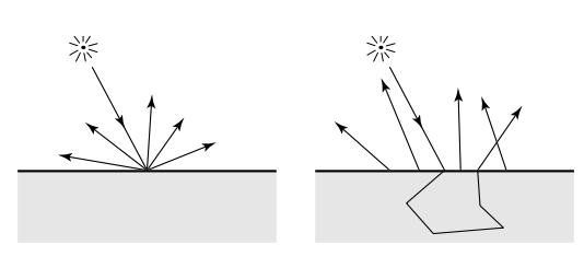
We attempted to extend the raytracer project and implement subsurface scattering in order to render translucent materials. Translucent materials do not reflect light in all directions when light hits it, some of the light goes within the material and scatters within, being emitted at other nearby locations. The Jensen paper proposes a combination of dipole model (modeling diffusion) and a single scattering model.

Technical Approach

Dipole Model

From the original (Jensen 2001) paper: the irradiance value is
$S(x_{i},\omega_{i};x_{o},\omega_{o}) = S_{d}(x_{i},\omega_{i};x_{o},\omega_{o}) + S^{(1)}(x_{i},\omega_{i};x_{o},\omega_{o})$. The complete BSSRDF model is approximated by a sum of two terms, a diffusion term and a single-scattering term:
$L(x_{o},\omega_{o})=\int_{A}\int_{\Omega}L_{i}(x_{i},\omega_{i})S(x_{i},\omega_{i};x_{o},\omega_{o})\cos(\theta)d\omega dA$, $S_{d}(x_{i},\omega_{i};x_{o},\omega_{o})=\frac{1}{\pi}F_{t}(x_{i},\omega_{i})R_{d}(\|x_{i} - x_{o}\|)F_{t}(x_{o},\omega_{o})$. To approximate diffusion, an incoming ray is transformed into a dipole source with a real and virtual light source. $F_{t}$ is the Fresnel term for dielectric surfaces, $R_{d}$ is diffuse reflectance due to dipole source that decays exponentially as a function of $r$ (distance from the raytraced point).

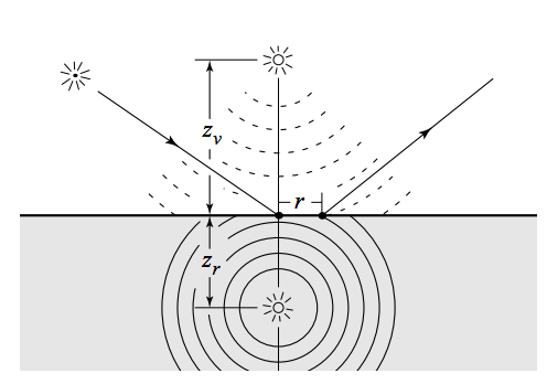
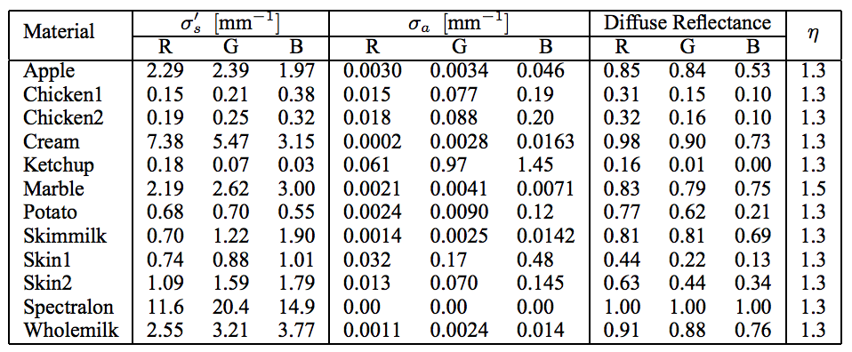
Diffuse BSSRDF term: $R_{d}(r)=\frac{\alpha}{4\pi}[z_{r}(\sigma_{tr}d_{r}(r)+1)\frac{e^{-\sigma_{tr}d_{tr}(r)}}{d_{r}^{3}(r)}+z_{v}(\sigma_{tr}d_{v}(r)+1)\frac{e^{-\sigma_{tr}d_{v}(r)}]}{d_{v}^{3}(r)}$ where $\sigma_{tr}=\sqrt{3\sigma_{a}((1-g)\sigma_{s}+\sigma_{a})}$ is the effective extinction coefficient, $d_{r}(r) = \sqrt{z_{r}^{2}+r^{2}}$, $d_{v}(r)=\sqrt{z_{v}^{2}+r^{2}}$ are real and virtual light refractions, $z_{v}=\frac{1}{\sigma_{t}'},z_{r}=z_{v}+\frac{4}{3\sigma_{t}'}\frac{1+F_{dr}}{1-F_{dr}}$ are real and virtual light source distances, and $F_{dr}=-\frac{1.44}{\eta^{2}}+\frac{0.71}{\eta}+0.668+0.0636\eta$ is the rational approximation of diffuse reflectance where $\sigma_s$ is the scattering coefficient, $\sigma_t$ is the extinction coefficient and $\eta$ is the index of refraction. These constants are all known properties of the material that must be chosen beforehand. The table of coefficients in the Jensen paper lists the coefficients for many materials.

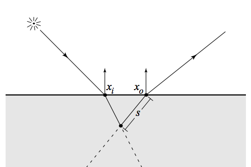
Single Scatter term: $L_{o}^{(1)}(x_{o},\omega_{o}) = \frac{\sigma_{s}(x_{o})}{\sigma_{tc}}F_{t}(\eta^{-1},\omega_{o})F_{t}(\eta,\omega_{i})p(\omega_{i} \cdot \omega_{o}) e^{-s_{i}'\sigma_{t}(x_{i})}e^{-s_{o}'\sigma_{t}(x_{o})} L_{i}(x_{i}, \omega_{i})$ where $p$ is the Henyey-Greenstein phase function $p(\theta)=\frac{1}{4\pi}\frac{1-g^{2}}{[1+g^{2}-2g\cos(\theta)]^{3/2}}$. The $\sigma$ functions depend on the point on entry and the point of outgoing radiance too. Single scattering occurs when the refracted incoming and outgoing rays intersect and is computed as an integral over path lengths. $\sigma_{t}=\sigma_{s}+\sigma_{a}$ is the extinction coefficient and $\sigma_{tc}=\sigma_{t}(x_{o})+\frac{|n_{i}\cdot\omega_{o}'|}{|n_{i}\cdot\omega_{i}'|}\sigma_{t}(x_{i})$ is the combined extinction coefficient. $s_{o}'=\frac{\log(\xi)}{\sigma_{t}(x_{o})}$ is the sampled distance along the refracted outgoing ray and $s_{i}'=s_{i}\frac{\|\omega_{i}\cdot n_{i}\|}{\cos(\theta_{i}')}$.

The formulas are all fine and dandy, but you’ll notice that these formulas all depend on the initial point of intersection and a second point nearby on the surface $(x_{o}, x_{i})$. This is due to the fact that the luminance of translucent materials depends on that point and the nearby area surrounding it. To do that, we need to sample points along the surface in the nearby area around the intersect point.

Sampling Positions

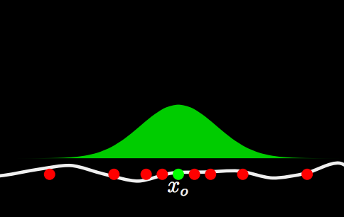
The original (Jensen 2001) paper mentioned a sampling method to generate samples in a disk around the original intersection point from the camera to the scene. This method is great for flat surfaces, but the vast majority of samples will not lie on the surface if the surface is curvy. Other sources mention augmenting this method by generating points in a disk and then shooting them in the direction of the normal vector at the original intersection point, checking for an intersection with the scene and taking those points as the points we sample.

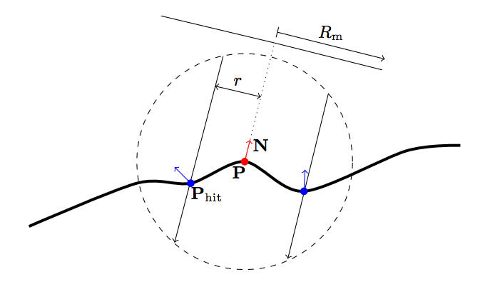
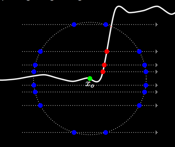
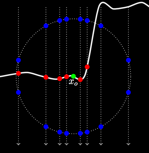
(Kulla 2013) mentioned a novel technique where instead of just sampling on a disk, we sample on three different axis (one of which is the normal vector direction at the point of intersection) within a sphere. We bound a sphere of radius $R_{max} = \sqrt{v/12.46}$ and probe rays along three different axis and mark any intersection points within the sphere as the points that we draw and measure the effective radiance from.

Importance Sampling

(Kulla 2013) mentioned that the final contribution of each point is modulated by $\frac{R_{d}(\|P_{hit}-P\|)}{pdf_{disk}(r)}\frac{1}{|V \cdot N_{hit}|}$ where $pdf_{disk}(r)=R_{d}(r)/(1-e^{-R_{m}^{2}/2v})$, $r(\xi) = \sqrt{-2v\log(1-\xi(1-e^{-R_{m}^{2}/2v}))}$ and $v = \frac{1}{2\sigma_{tr}}$ is the formula for sampling random points on a disk. We also choose the axis to sample at a ratio of 2:1:1 for the normal vector direction versus the two other axis directions and also take that into account when modulating points by the pdf.

Framework Changes

We had to modify the .dae file by adding parameters, so the raytracer knew the coefficient values it needed to render the material properly. These properties were inserted XML-style into the files like:

<technique profile="CGL"> <bssrdf> .. </bssrdf> </technique>
  

We edited the collada file collada.cpp to be able to fetch the new data written into the .dae files:

if (type == "bssrdf") {
    XMLElement *e_eta = get_element(e_bsdf, "eta");
    .....
  }

We added a BSSRDF class to bsdf.h/bsdf.cpp to figure out which materials have that BSDF. Also added an is_bssrdf() variable to easily tell the class. If so, instead of estimating direct or indirect illumination, we call the subsurface() function in the pathtracer which adds both L for single scattering and diffusion.

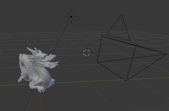
We also modified the .dae models with Blender, changing the light sources to point lights, removing the pedestal, and moving the lights to favorable positions.

Workflow

With the following methods and ideas all explained, we describe the resulting workflow of the ray tracer.

Upon an intersection of a ray traced from the camera to the scene, we call the subsurface() method which calculates the diffusion $S_{d}$ and the single-scattering $S^{(1)}$ terms. For $S_{d}$ it calculates all the necessary constants and Fresnel terms $F_{t}$. It generates a ray to probe into the bounding sphere of radius $R_{max}$ and takes the intersection of the point with the same BSSRDF material and calculates $R_{d}$ based on the two locations $(x_{i},x_{o})$. From the area intersection point, it sends a shadow ray to sample the amount of light on that point and then we aggregate all the terms to calculate $S_{d}$ and divide by the pdf. For $S^{(1)}$, we take the traced ray and refract it within the material and choose a random distance along this refracted ray according to exponential pdf. That will be our new sampled point, which we shoot a shadow ray in the direction of the light at which it intersects with the material again and we have our new sampled point on the surface. We have enough information to evaluate the expression for $S^{(1)}$, along with all the constants and parameters. With enough samples we approximate the ground truth value of the scene.

Problems

• Most of the time was spent trying to figure out what to do. The (Jensen 2001) paper was not clear at all about what to do, and we had to consult many different resources that tried to explain what the formulas actually meant when implemented rather than some theoretical integral or implicit formulation from the paper.

• We spent nearly a whole week with an image that didn’t look any different than the regular diffuse case besides being very dark. We later realized that the subsurface scattering model depends on the area nearby the intersection point and we were taking light samples and shooting shadow rays from the original intersection point rather than the nearby points in the area. We also had another bug with the wrong origin point when shooting the shadow ray since we were repeating code.

• Since the BSSRDF class extended the virtual BSDF class from the existing raytracer and we added new methods into the BSSRDF class since we had a separate function for subsurface() scattering we thought we had to add every additional method in BSSRDF to the main virtual BSDF class and put them in the other classes that extend BSDF too. This was a lot of work, but we realized that since we can detect whether a BSDF is BSSRDF or not with the is_bssrdf() variable we included, we just left that as an if case and casted the BSDF into BSSRDF so we could call the additional functions. We are quite proud of this clever trick.

  if (isect.bsdf->is_bssrdf()) {
  BSSRDF const bssrdf = (BSSRDF const ) isect.bsdf;
  bssrdf->bssrdf_methods();
  ….
  }

• We initially had parameter issues regarding the scale of the constants (because the values listed in the table were in units of $mm^{-1}$ whereas the scene wasn’t) that made the material too translucent to the point that it looked like ice or glass.

Results

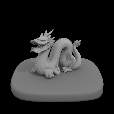
This is what the dragon looks like under regular diffuse lighting.

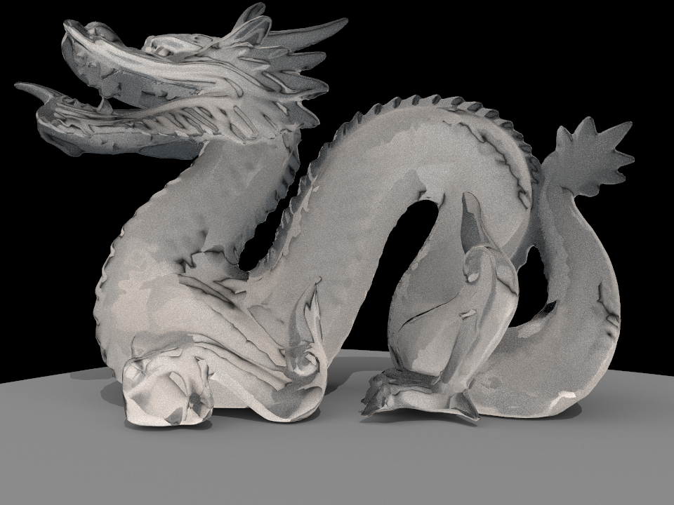
This is what the dragon looks like when we had the issue with the scale of coefficients that made the dragon look like ice or glass.

Below are the three resulting images and what the scene file looked like in Blender.

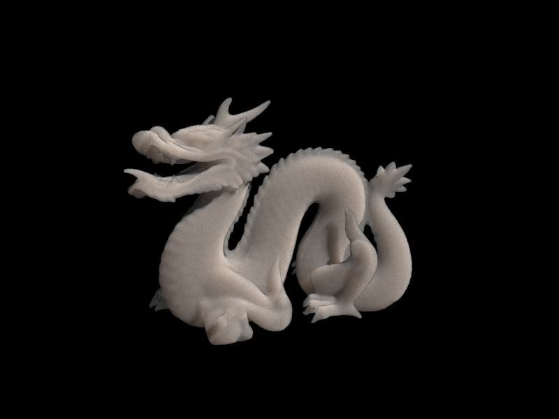
Dragon (Marble)

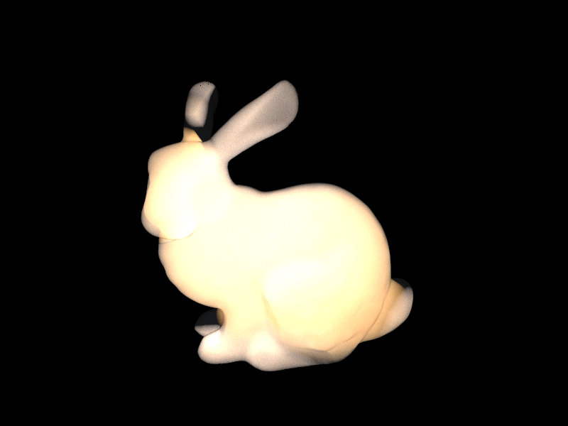
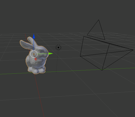
Bunny (Chicken)

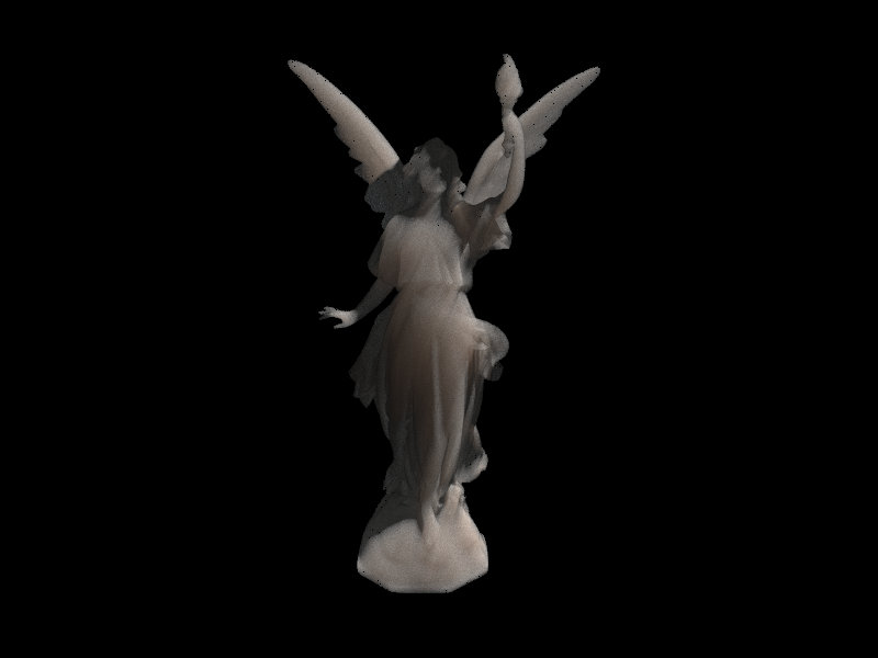
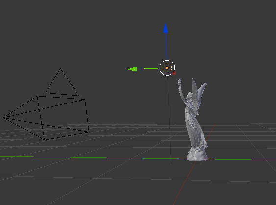
Lucy (Marble)

References

A Practical Model for Subsurface Scattering Light Transport (Jensen 2001)
Fast BSSRDF (Jensen 2002)
BSSRDF Summary (Koutajoki 2002)
Implementing a Skin BSSRDF (Hery 2003)
BSSRDF Notes (Scukanec 2004)
BSSRDF Importance Sampling (Kulla 2013)
Approximate BSSRDF (Christensen 2015)

Contributions

Juchan: .dae file modification and integration with pathtracer. Coding.
Kai: Reference gathering and understanding the math and models. Coding.

We coded most of the project together in the same room.

Video and Slides

Slides
Video Explaining Slides